TimesFM-3: What Changed in Google's Time-Series Foundation Model?
TimesFM-3: What Changed in Google’s Time-Series Foundation Model?
From single-series extrapolation to native multivariate forecasting with dynamic future awareness.
Google has released TimesFM-3, the third generation of its pretrained time-series foundation model family.
While incremental accuracy improvements are common across model iterations, TimesFM-3 introduces a fundamental architectural departure from earlier generations: it transitions from univariate extrapolation (predicting a single isolated sequence) to native multivariate forecasting with full support for known future signals (covariates) and probabilistic uncertainty quantiles.
To evaluate these capabilities first-hand, I set up a synthetic retail forecasting experiment in Google Colab, testing how TimesFM-3 performs across univariate, multivariate, and future-covariate settings.
1. What is TimesFM?
Time-series forecasting has historically been dominated by task-specific model pipelines: classical statistical methods (ARIMA, ETS), gradient-boosted trees (LightGBM, XGBoost) with manual lag engineering, and deep neural architectures (LSTM, DeepAR, PatchTST) trained from scratch on individual datasets.
Traditional Workflow:
Raw Time Series Data -> Dataset-Specific Feature Eng -> Train Model from Scratch -> Forecast
Google’s TimesFM (Time-Series Foundation Model) introduced a zero-shot alternative inspired by Large Language Models: pretrain a large decoder-only Transformer on a massive corpus of diverse time-series data once, and perform zero-shot inference on entirely unseen domains without task-specific fine-tuning or retraining.
The initial TimesFM model (2024) demonstrated that patching and self-attention mechanisms could scale effectively to continuous temporal sequences across 100 billion real-world time points.
2. The Univariate Limitation of Previous Versions
Despite strong zero-shot performance on standard benchmarks, TimesFM versions up to 2.5 shared a core architectural constraint: they were strictly univariate.
In a univariate framework, the model assumes the future trajectory of a target variable is solely a function of its own historical values:
Past Sales: [100, 110, 120, 115, 130] -> Future Sales: [?]
In real-world physical, operational, and commercial systems, this assumption rarely holds. Consider daily retail sales:
- Customer foot traffic drives store visits.
- Marketing promotions and discounts create demand spikes.
- Temperature and weather fluctuations shift consumer preferences.
- Competitor pricing and public holidays alter buying patterns.
When a model only observes historical sales, it is forced to guess upcoming inflections without seeing the causal drivers that create them. This is the exact limitation TimesFM-3 addresses.
3. What is New in TimesFM-3? Previous vs. This Version
TimesFM-3 is not simply a larger version of TimesFM-2.5. Google re-engineered the input representation, attention mechanics, and decoding pipeline to build a natively multivariate system.
3.1 Univariate Modeling vs. Native Multivariate Modeling
Previous Versions (TimesFM 1.0 & 2.5): Each time series had to be forecasted in complete isolation. If you had sales, foot traffic, and temperature, you had to run three separate univariate models. The model could not share information across related channels.
TimesFM-3: The model natively accepts multiple continuous channels simultaneously. It jointly forecasts target variables while learning cross-series correlations and co-movement dynamics:
Sales History + Traffic History + Temperature History -> Joint Future Forecast
If historical observations show that an increase in foot traffic precedes a surge in revenue, TimesFM-3 uses that cross-series relationship directly during inference.
3.2 Blind Extrapolation vs. Dynamic Future Covariates
Previous Versions: Earlier models could only extrapolate from past data. They had no mechanism to accept information about planned future events.
TimesFM-3: TimesFM-3 introduces support for two distinct types of exogenous variables:
- Past Covariates: Signals observed historically whose future values are unknown at forecast time (for example, recorded local temperature or past foot traffic).
- Dynamic / Past-Future Covariates: Deterministic signals known both historically and across the entire future forecast horizon (for example, planned discount promotions, scheduled holidays, maintenance outages, or marketing ad schedules).
This changes the forecasting task from: “What usually happens after this historical pattern?”
to: “What is likely to happen next, given the future events and promotions we have already scheduled?“
3.3 1D Temporal Attention vs. 2D Temporal-Variate Attention
Previous Versions: TimesFM-1.0 and 2.5 used standard 1D self-attention across the time dimension of a single series.
TimesFM-3: TimesFM-3 structures the input into a 2D patch grid (Variables x Time) and alternates between two orthogonal attention mechanisms:
- Temporal Attention: Computes attention across the time dimension for each variable independently, capturing seasonality, trends, and lag structures.
- Variate Attention: Computes cross-attention across different variables at corresponding time steps, capturing cross-signal dependencies and covariate interactions without quadratic complexity explosion.
3.4 Autoregressive Sequential Patches vs. Single-Pass Non-Autoregressive Decoding
Previous Versions: Earlier TimesFM models generated long-horizon forecasts autoregressively (patch-by-patch). This sequential generation introduced higher inference latency and allowed prediction errors in earlier patches to cascade into subsequent steps.
TimesFM-3: TimesFM-3 adopts Contiguous Patch Masking to generate the complete forecast horizon in a single forward pass. This non-autoregressive decoding strategy significantly speeds up batched inference while eliminating rollout drift.
3.5 Pretraining Scale and Model Capacity
- TimesFM-1.0: 200M parameters pretrained on approximately 100 billion real-world time points.
- TimesFM-2.5: Refined 200M parameter backbone with improved zero-shot univariate accuracy.
- TimesFM-3: Scaled to 330M parameters and pretrained on a corpus exceeding 1 trillion time points from diverse real-world domains and synthetic generators.
3.6 Deterministic Point Forecasts vs. 9-Quantile Probabilistic Distributions
While earlier versions primarily focused on point predictions (with experimental quantile support in later 2.5 iterations), TimesFM-3 natively includes a multi-quantile output head providing 9 target percentiles (10th, 20th, …, 90th). This allows users to inspect the full risk envelope for safety stock, capacity planning, and operational risk assessment.
4. TimesFM Family Evolution at a Glance
| Capability | TimesFM (Original) | TimesFM-2.5 | TimesFM-3 |
|---|---|---|---|
| Zero-Shot Forecasting | Yes | Yes | Yes |
| Primary Mode | Univariate | Univariate | Multivariate and Univariate |
| Auxiliary Covariates | No | No | Past and Future Dynamic Covariates |
| Attention Architecture | 1D Temporal | 1D Temporal | 2D Temporal-Variate Alternating |
| Decoding Strategy | Autoregressive Patches | Autoregressive Patches | Single-Pass Non-Autoregressive |
| Probabilistic Quantiles | Basic | Point and Quantile | Full 9-Quantile Distribution (10th to 90th) |
| Parameters | 200M | ~200M | 330M |
| Pretraining Corpus | 100B time points | ~200B time points | 1T+ time points |
5. Empirical Experiment: Synthetic Retail Forecasting
To inspect how TimesFM-3 behaves in practice, I generated a 300-day synthetic retail dataset containing four co-evolving signals:
- Sales (Target): Driven by traffic, temperature, promotions, and stochastic noise.
- Customer Foot Traffic: Weekly cyclic seasonality with seasonal shifts.
- Temperature: Annual sinusoidal wave (scaled by 20 for variance).
- Promotions: Scheduled discount campaigns (active in repeated pulses).
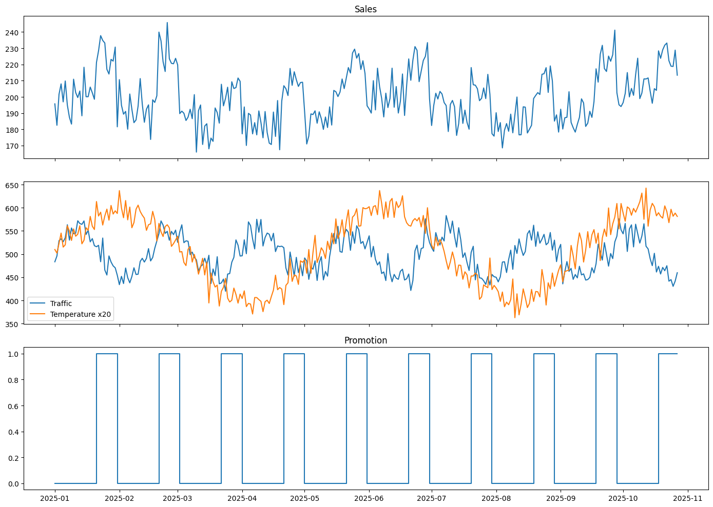
Figure 1: Generated 300-day multi-signal retail environment showcasing sales, traffic, temperature, and cyclic promotion schedules.
The repeated rectangular promotion pulses represent a known operational schedule, making it an ideal test case for evaluating future covariate utilization.
6. Experimental Setup: 270-Day Context & 30-Day Horizon
We split the 300 daily observations into an out-of-sample evaluation setup:
- Context Window: The first 270 days (Day 1 to Day 270) are provided as historical inputs.
- Forecast Horizon: The final 30 days (Day 271 to Day 300) are withheld for out-of-sample evaluation.
The final 30 days of sales are withheld from the model during inference. After generating the forecast, we compare the prediction against the actual held-out sales trajectory.
7. Experiment 1 vs. Experiment 2: Univariate vs. Multivariate Forecasting
In the first test, TimesFM-3 operated in univariate mode, receiving only historical sales. In the second test, TimesFM-3 operated in multivariate mode, receiving sales, traffic, temperature, and promotion channels jointly.
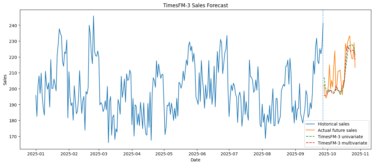
Figure 2: Historical context (270 days) vs. 30-day forecast horizon comparing univariate and multivariate TimesFM-3 predictions against actual sales.
Key Observations:
- In univariate mode, the model captures the overall level and baseline periodicity but cannot anticipate demand inflections triggered by external events.
- In multivariate mode, the model leverages historical correlations across foot traffic and temperature to generate a more responsive forecast.
8. Experiment 3: Leveraging Known Future Promotion Covariates
In the third experiment, we provided the known future promotion schedule across the 30-day forecast horizon as a dynamic covariate.
In real operations, a business already knows its promotional calendar. Supplying this schedule allows the model to condition its forecast directly on planned marketing events.
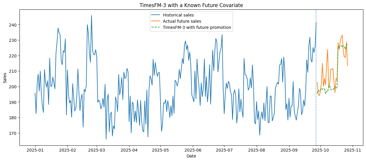
Figure 3: TimesFM-3 forecast with known future promotion covariates, accurately matching the demand surge during the scheduled promotion window.
Key Takeaway:
When provided with the future promotion schedule, TimesFM-3 immediately lifts its sales forecast specifically during the promotion window. The model does not need to guess whether an event will happen; it only estimates the magnitude of the response based on historical interactions.
9. Probabilistic Uncertainty Estimation
Forecasting a single deterministic trajectory is often insufficient for business planning. TimesFM-3 outputs quantile intervals across the 10th to 90th percentiles:
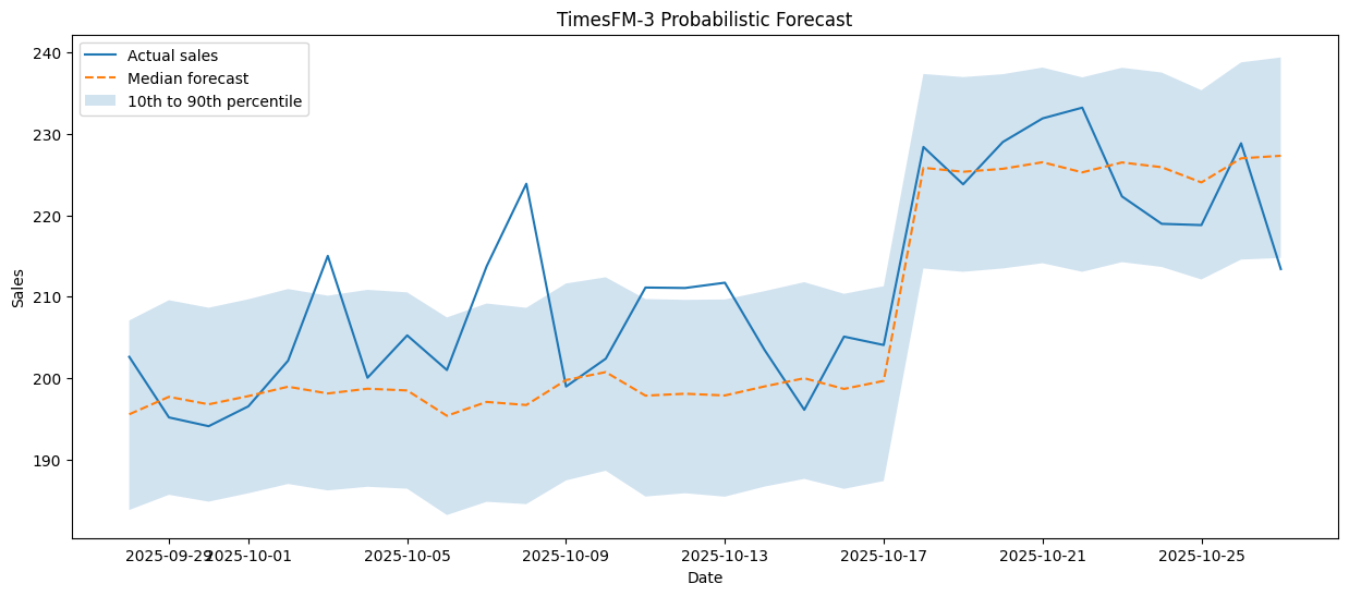
Figure 4: TimesFM-3 probabilistic forecast showing median trajectory alongside the 10th-to-90th percentile prediction interval.
The shaded band provides an uncertainty envelope:
- The dashed line represents the median forecast.
- The shaded region illustrates the range between the 10th and 90th percentiles.
- During promotion windows, the entire uncertainty envelope shifts upward, reflecting both higher expected volume and increased variance.
10. Benchmark Performance & Google Research Findings
Google evaluated TimesFM-3 across major standardized time-series benchmarks, including GIFT-Eval, FEV-Bench, and TIME:
- GIFT-Eval: TimesFM-3 achieved the top average rank among evaluated pretrained foundation models for both point and probabilistic forecasting.
- FEV-Bench: Demonstrated competitive advantages against recent multivariate foundation models such as Chronos-2 and the Toto 2.0 family.
- Univariate vs. Multivariate: Google reports that TimesFM-3 performs strongly even in standalone univariate mode due to its 330M parameter capacity, while its multivariate mode delivers additional performance gains whenever auxiliary channels exist.
11. Hands-On Google Colab Notebook
You can inspect the complete implementation, run the synthetic data generator, and test TimesFM-3 inference directly in Google Colab:
Open TimesFM-3 Google Colab Notebook
The notebook includes:
- Environment setup and TimesFM-3 installation
- Multi-channel synthetic retail signal generation
- Univariate vs. multivariate forecast execution
- Future covariate conditioning and quantile visualization
- Out-of-sample forecast plotting
12. Summary and Progression
The evolution of Google’s time-series foundation models represents a clear shift in capability:
TimesFM (2024): 200M params, 100B points -> “Can foundation models do zero-shot forecasting?”
TimesFM-2.5: Improved architecture -> “Can we refine zero-shot univariate accuracy?”
TimesFM-3: 330M params, 1T+ points -> “Can we model complex multi-signal dynamic systems?”
The primary advancement in TimesFM-3 is not simply scale. It is the ability to model co-evolving signals and incorporate scheduled future events in a single forward pass, aligning foundation models with how real-world forecasting problems are structured.
Sources & References
- Google Research: TimesFM-3: A Zero-Shot Foundation Model for Multivariate Forecasting
- Google Research: A Decoder-Only Foundation Model for Time-Series Forecasting
- Google Research: Time-Series Foundation Models Can Be Few-Shot Learners
- GitHub Repository: google-research/timesfm